Decision Trees
-
represent discrete-valued functions
-
instances described by attribute-value pairs
-
can represent disjunctive expressions (unlike version spaces)
-
robust to noisy training data (unlike version spaces)
-
can handle missing attributes (unlike version spaces)
-
one of the most popular and practical methods of inductive
learning
-
Idea: ask a series of questions about the attributes
of an instance in order to arrive at the correct classification
Some successful applications of decision trees:
-
classifying patients by disease
-
classifying equipment malfunctions by cause
-
classifying loan applications by level of risk
-
classifying astronomical image data
-
learning to fly a Cessna by observing pilots on a simulator
- data generated by watching three skilled human pilots performing a fixed
flight plan 30 times each
- new training example created each time pilot took an action by setting a
control variable such as thrust or flaps
- 90,000 training examples in all
- each example described by 20 attributes and labelled by the action taken
- decision tree learned by Quinlan's C4.5 system and converted to C code
- C code inserted into flight simulator's control loop so that it could fly
the plane by itself
- program learns to fly somewhat better than its teachers
- generalization process cleans up mistakes made by humans
- Reference: Sammut, C., Hurst, S., Kedzier, D., and Michie, D. (1992).
Learning to fly. In Proceedings of the Ninth International Conference on
Machine Learning, Aberdeen. Morgan Kaufmann.
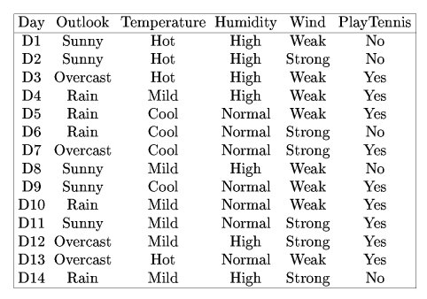
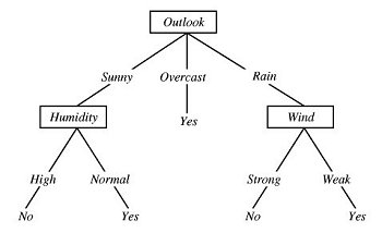
Example: Decision tree for
the concept PlayTennis

<Outlook=Sunny, Temp=Hot, Humidity=High,
Wind=Strong> classified as No
In general, decision trees are disjunctions of conjunctions
of constraints on attribute values.
Above tree is equivalent to the following logical expression:
(Outlook=Sunny ^ Humidity=Normal)
v (Outlook=Overcast) v (Outlook=Rain ^ Wind=Weak)
Constructing Decision Trees
Idea: Determine which attribute of the examples makes
the most difference in their classification and begin there.
Inductive bias: Prefer shallower trees that ask fewer
questions.
Example: Boolean function: first bit or second bit on.
| Instance |
Classification |
| A 000 |
- |
| B 001 |
- |
| C 010 |
+ |
| D 011 |
+ |
| E 100 |
+ |
| F 101 |
+ |
| G 110 |
+ |
| H 111 |
+ |
We can think of each bit position as an attribute (with
value on or off). Which attribute divides the examples
best?
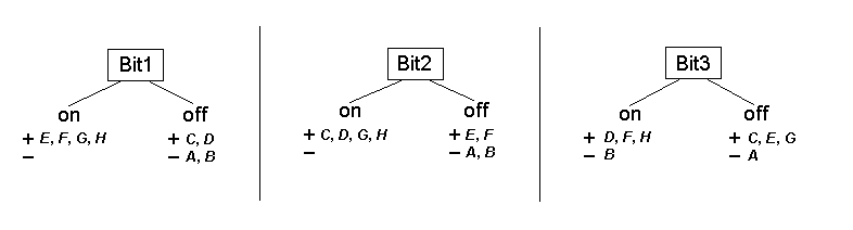 Bits 1 and 2 are equally good starting points, but Bit 3
is less desirable.
Bits 1 and 2 are equally good starting points, but Bit 3
is less desirable.
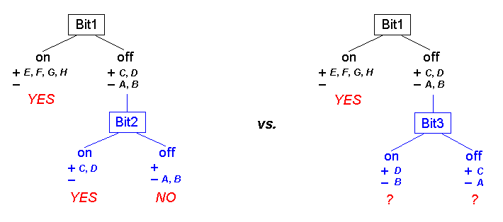
Let's start with Bit1. The left branch of this tree
is complete -- no more work is necessary. Need to complete right
branch.
Consider Bit2 vs. Bit3. Bit2 is better:
This decision tree is equivalent to the following logical
expression:
Bit1(on) v (Bit1(off) ^ Bit2(on))
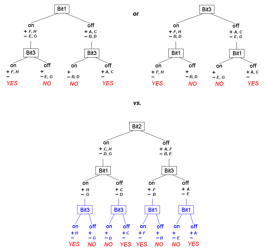
Example: Boolean function: first and last bits equal.
| Instance |
Classification |
| A 000 |
+ |
| B 001 |
- |
| C 010 |
+ |
| D 011 |
- |
| E 100 |
- |
| F 101 |
+ |
| G 110 |
- |
| H 111 |
+ |
Bit1, Bit2, and Bit3 look equally good at the beginning,
but it turns out that Bit2 is actually worse in the long run:
These trees are equivalent to the following logical expressions:
(Bit1(on) ^ Bit3(on)) v (Bit1(off)
^ Bit3(off))
(Bit3(on) ^ Bit1(on)) v (Bit3(off)
^ Bit1(off))
(Bit2(on) ^ Bit1(on) ^ Bit3(on))
v (Bit2(on) ^ Bit1(off) ^ Bit3(off)) v (Bit2(off) ^ Bit3(on) ^ Bit1(on))
v (Bit2(off) ^ Bit3(off) ^ Bit1(off))
Constructing a decision tree in this manner is a hill-climbing
search through a hypothesis space of decision trees.
Tree with Bit2 attribute at root corresponds to a local
(suboptimal) maximum.
How to determine best attribute in general?
Use entropy to compute information gain.
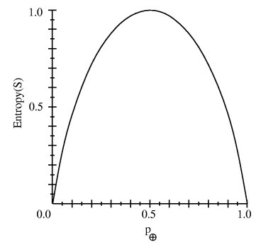
Entropy measures heterogeneity of a set of examples.
Entropy(S) = -p(+)
log2 p(+)
- p(-)
log2 p(-)
where p(-)
and p(+) are the proportion
of positive and negative examples in S.
Example:
Entropy([9+, 5-])
= - (9/14) log2
(9/14) - (5/14) log2
(5/14) = 0.940
Entropy = 0 implies that all examples in S have the same
classification.
Entropy = 1 implies equal numbers of positive and negative
examples.
Interpretations of Entropy:
-
number of bits needed to encode the classification of an
arbitrary member of S chosen at random
-
uncertainty of classification of an arbitrary member of S
chosen at random
General case: n possible values for classification
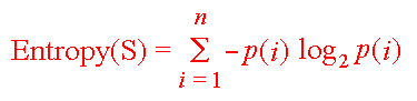
Range of possible values: 0 <
Entropy(S) < log2 n
Information gain measures reduction in entropy
caused by partitioning examples according to a particular attribute.
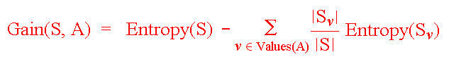
where Values(A) is the set of possible values for attribute
A and Sv is
the subset of examples with attribute A = v.
The sum term is just the weighted average of the entropies
of the partitioned examples (weighted by relative partition size).
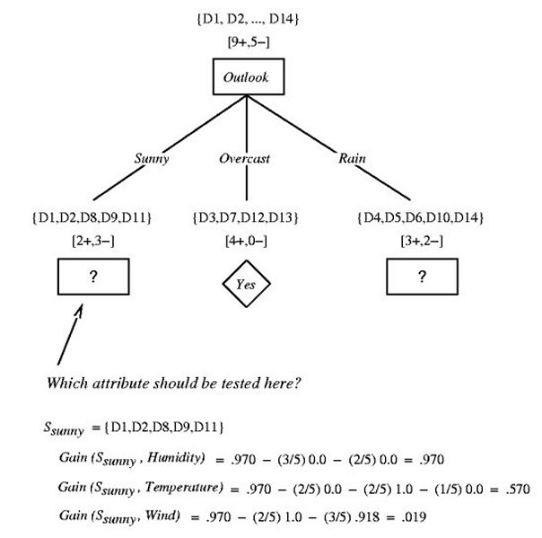
Example: Learning the concept of PlayTennis
Values(Wind) = { Weak, Strong }
S: [9+, 5-]
SWeak:
[6+, 2-]
SStrong:
[3+, 3-]
Gain(S, Wind) = Entropy(S) -
(8/14) Entropy(SWeak)
-
(6/14) Entropy(SStrong)
= 0.940 - (8/14) 0.811 -
(6/14) 1.00
= 0.048
Humidity versus Wind:
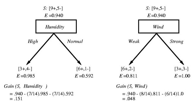
Similar computations for Outlook and Temp yield:
-
Gain(S, Outlook) = 0.246 <---
chosen attribute
-
Gain(S, Humidity) = 0.151
-
Gain(S, Wind) = 0.048
-
Gain(s, Temp) = 0.029
Resulting partially-constructed tree:
Decision Tree Learning Algorithm
DTL(Examples, TargetAttribute, Attributes)
/* Examples are the training examples. TargetAttribute
is the attribute whose value is to be predicted by the tree. Attributes
is a list of other attributes that may be tested by the learned decision
tree. Returns a decision tree that correctly classifies the given
Examples.
*/
-
create a Root node for the tree
-
if all Examples are positive, return
the single-node tree Root, with label = Yes
-
if all Examples are negative, return
the single-node tree Root, with label = No
-
if Attributes is empty, return the single-node
tree Root, with label = most common value of TargetAttribute
in Examples
-
else begin
-
A <--
the attribute from Attributes with the highest information gain
with respect to Examples
-
Make A the decision attribute for Root
-
for each possible value v of A {
-
add a new tree branch below Root, corresponding to
the test A = v
-
let Examplesv be the subset of Examples
that have value v for attribute A
-
if Examplesv is empty then
add a leaf node below this new branch with label = most
common value of TargetAttribute in Examples
else
add the subtree DTL(Examplesv, TargetAttribute,
Attributes - { A })
}
end
|
DTL performs hill-climbing
search using information gain as a heuristic.
Characteristics of DTL
-
hypothesis space is complete: every finite discrete-valued
function can be represented by some decision tree, so target function is
always in H
-
maintains only a single hypothesis -- no backtracking possible
-
cannot determine how many other trees are consistent with
examples
-
cannot pose new queries that maximize information
-
uses all training examples at each step to refine
hypothesis => much less sensitivity to noise/errors
-
inductive bias: shorter trees preferred; trees with high
information gain attributes closer to root preferred
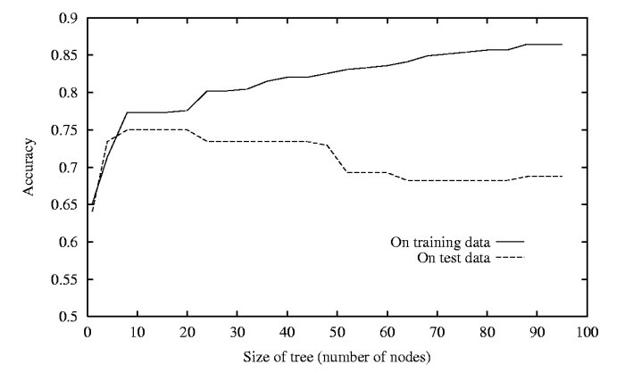
Overfitting
-
Hypothesis h overfits the data if there exists
h'
with greater error than h over training examples but less error
than h over entire distribution of instances
-
Serious problem for all inductive learning methods
-
Trees may grow to include irrelevant attributes (e.g.,
Date)
-
Noisy examples may add spurious nodes to tree
- Effects of overfitting
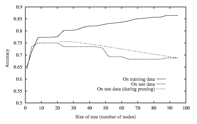
Decision Tree Pruning
-
Reduced-error pruning
1. divide data into training set and
validation
set
2. build a decision tree using the training set, allowing
overfitting to occur
3. for each internal node in tree:
-
consider effect of removing subtree rooted at node, making
it a leaf, and assigning it majority classification for examples at that
node
-
note performance of pruned tree over validation set
4. remove node that most improves accuracy over validation
set
5. repeat steps 3 and 4 until further pruning is harmful
-
Effects of reduced-error pruning
-
Rule post-pruning
-
infer decision tree, allowing overfitting to occur
-
convert tree to a set of rules (one for each path in tree)
-
prune (generalize) each rule by removing any preconditions
(attribute tests) that result in improving its accuracy over
the validation set
-
sort pruned rules by accuracy, and consider them in this
order when classifying subsequent instances
-
example:
IF     (Outlook = Sunny) ^ (Humidity = High)
THEN   PlayTennis = No
Try removing (Outlook = Sunny) condition or (Humidity =
High) condition from the rule and
select whichever pruning step leads to the biggest improvement in accuracy on
the validation set (or else neither if no improvement results).
-
advantages of rule representation:
- each path's constraints can be pruned independently of other paths in the
tree
- removes distinction between attribute tests that occur near the root and
those that occur later in the tree
- converting to rules improves readability
Continuous-Valued Attributes
Dynamically define new discrete-valued attributes
that partition the continuous attribute into a discrete set of intervals
Example: Suppose we have training examples with
the following Temp values:
| Temp |
40 |
48 |
60 |
72 |
80 |
90 |
| PlayTennis |
No |
No |
Yes |
Yes |
Yes |
No |
Split into two intervals: Temp < val
and Temp > val
This defines a new boolean attribute Temp>val
How to choose val threshold?
Consider boundary cases val = (48+60)/2 = 54 and
val
=
(80+90)/2 = 85
Possible attributes: Temp>54 ,
Temp>85
Choose attribute with largest information gain (as
before): Temp>54
This approach can be generalized to multiple thresholds.
Missing Attributes
-
If a training example in S is missing an attribute value
at some node during tree construction, just "guess" an appropriate value
by filling in with the most common value among other examples at that node.
-
If a novel instance is missing an attribute value that needs
to be tested, determine possible values for that attribute and ask decision
tree for classification assuming each possible value. Then return
a final classification based on the individual classifications weighted
by the probabilities of each attribute value.
Gain Ratio and Split Information
-
Variant of Gain heuristic that penalizes attributes that split
the data into many small groups (e.g., Date).
-
GainRatio = Gain / SplitInformation
-
SplitInformation = Entropy of examples with respect to
attribute values.
Reference: Machine Learning, Chapter 3, Tom M. Mitchell, McGraw-Hill,
1997.