Due by class time Monday, April 24
You may work with a partner on this assignment if you wish.
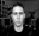
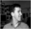
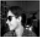
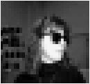
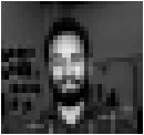
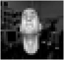
For this assignment, you will experiment with training neural networks to recognize images of faces. Each image will be a 32 × 30 array of grayscale pixels, which we'll represent as a list of 960 real numbers ranging from 0.0 (black) to 1.0 (white). This format is suitable for processing by neural networks. Some example face images are shown below:
We will use several datasets for this assignment:
all-images.dat is a file of 300 face images. Each image shows a person looking either left, right, forward, or up, and either wearing sunglasses or not. Each image is encoded as a vector of 960 values between 0.0 and 1.0, one image per line.
pose-targets.dat contains 300 binary target patterns of the form [left right forward up] indicating the pose of each person in all-images.dat. For example, the first line of pose-targets.dat is 0 0 1 0, meaning that the image encoded on the first line of all-images.dat is looking forward.
forward-images.dat contains 156 images of people looking straight ahead (with or without sunglasses on).
eye-targets.dat contains 156 target classifications for the images in forward-images.dat indicating whether each person is wearing sunglasses or not. Each line is either 1 (wearing sunglasses) or 0 (not wearing sunglasses).
name-targets.dat contains 156 target patterns indicating the name classification of each person in forward-images.dat. Each target is a binary vector of length 20 containing a single 1, representing the following names in order from left to right: Albert, Bob, Carl, David, Evan, Fred, George, Herbert, Ian, John, Kyle, Mike, Neil, Paul, Robert, Sarah, Teresa, Valerie, Walter, Zach.
Finish Lab 12 first before starting on this assignment. The handwritten-digit recognizer we developed in lab will be similar in structure to the face recognizer.
Use faces.py as your starting point for the face recognizer. This code sets up a network for implementing a "sunglasses recognizer", using the face images in forward-images.dat and the target values in eye-targets.dat as training data. The network has 960 input units, 3 hidden units, and 1 output unit. Start the program in Python and look at some of the face images interactively, like you did in Lab 12 using the showPattern method. Also look at the corresponding target pattern for each image.
Before training the network, create graphical displays of the connections from the input layer to all three hidden units by typing:
n.showWeights('hidden', 0)
n.showWeights('hidden', 1)
n.showWeights('hidden', 2)
You should see what amounts to random noise. Now train the network and watch the weights change as learning progresses. Do the weights into the hidden units develop sensitivities to particular areas of the "visual field"? How many epochs does it take for the network to learn to classify all 156 images correctly?
Next, save the hidden unit activation patterns produced by the network for each image in a file, by typing n.saveHiddenReps('shades'). This runs through all of the images in the dataset and records the activation pattern produced on the hidden layer for each image in a file called shades.hiddens. These patterns can be thought of as the network's internal representations for each of the images learned during training.
Look at the resulting file of hidden patterns. Since these patterns are 3-dimensional, we can visualize them as points in "representation space" by using the Linux Gnuplot program. Start Gnuplot (just type gnuplot at the Linux prompt) and then type the command splot "shades.hiddens". Click and drag on the graph for a better view of the data. How well does the network appear to have learned to separate the "sunglasses" images from the "no sunglasses" images at the level of its internal representations? (To exit Gnuplot, just type Ctrl-D)
You may have noticed that saveHiddenReps also creates the file shades.labels. These labels correspond to the output classifications produced by the network for each of the input images, using the network's classify method. Currently, the classify method just returns None, so the labels file isn't really useful.
Add a method to the FacesNetwork class called targetCategory(target) that takes a binary target vector as input and returns a string representation of the target vector. For the sunglasses task, the string should be either 'sunglasses' for the target [1.0], or 'open' for the target [0.0]. Test your method as follows:
>>> print n.targetCategory(n.targets[0])
sunglasses
>>> print n.targetCategory(n.targets[50])
open
>>>
Likewise, add a method called classify(pattern) that takes an image as input and returns the output classification produced by the network for the image, represented as a string. For the sunglasses task, if the single output of the network is near 1 (within tolerance), 'sunglasses' should be returned; if the output is near 0 (within tolerance), 'open' should be returned; otherwise '???' should be returned.
Next, repeat steps 2 and 3 above. This time, after calling saveHiddenReps, the file shades.labels will contain the sunglasses/open classification labels produced by your classify method for each of the input images. Use Gnuplot to view the new hidden representations created by the network, and then create a cluster diagram of the data as follows. At the Linux prompt, type:
/common/cs/cs30/cluster shades.hiddens shades.labels > shades.out
This will create a file called shades.out that contains a hierarchical tree (drawn sideways) showing all of the points in shades.hiddens labeled by the corresponding strings in shades.labels. Each leaf of the tree corresponds to an internal hidden representation produced by the network in response to an image, and the leaf's label indicates the classification assigned to that image by the network (which could be right or wrong). The diagram shows how the network learned to structure its internal representations in attempting to solve the task. Compare this with the Gnuplot graph.
Copy your faces.py file to a new file called faces2.py, and use that for the next part.
Modify faces2.py to implement a network for recognizing poses: left, right, forward, or up, using the 300 images in all-images.dat and the targets pose-targets.dat. You'll need to change your representation of output patterns to binary vectors of length 4, but using three hidden units should still suffice for this task. You will also need to modify your targetCategory and classify methods appropriately. The classify method we used in Lab 12 may come in handy here. Also, write an evaluate() method that evaluates the network's performance on the testing images stored in self.testInputs (not the training images in self.inputs), like we did for Lab 12. In fact, you may want to reuse the code you wrote for the lab here.
Once everything is working, split the 300 images of the dataset into 180 training images (60% of the data) and 120 testing images (40% of the data) by typing n.splitData(60), and create weight displays for the three hidden units as before. Train the network and observe the weight changes that occur (warning: training will take longer due to the larger number of connections). Can you characterize the sensitivities developed by the hidden units to particular regions of the visual field? How many epochs are required on average for the network to fully learn the training set? After training, check the network's performance on the novel images in the testing set using your evaluate method. How many of the novel images does the network classify correctly? Does its ability to generalize seem better or worse than you expected? Save the weights of your trained network in a file by typing n.saveWeightsToFile('pose-recognizer.wts'), and then analyze the network's internal representations as before using Gnuplot and the clustering program.
Copy your faces2.py file to a new file called faces3.py, and use that for the next part.
Modify faces3.py to implement a 1-of-20 name recognizer. That is, implement a network that classifies images by name. For this task, use the 156 forward-looking images in forward-images.dat and the targets in name-targets.dat. Your network should have 20 output units (one for each possible name), and 9 hidden units. Split the images into equal-size training and testing sets (78 images each), and use a momentum of 0.8. After training, how well does the network perform on the testing set? What happens to the performance as you increase the number of hidden units? Can you find a combination of learning rate (epsilon) and momentum values and number of hidden units that leads to substantially better evaluation performance on the testing set? Save the weights of your best trained network in a file called name-recognizerN.wts, where N is the number of hidden units in your network.
Write up a summary of your experiments and turn this in during class. In addition, use /common/cs/submit/cs30-submit to submit the files listed below. Be sure to run this command from the directory containing your files.
If you have any questions, just ask!